Choose timezone
Your profile timezone:
In this example script we show how to use a Profile Cooker JSON file, the NEOTRANSP code, matlabVMEC, and the W7-X matlab tools to generate a fixed boundary VMEC input file with BEAMS3D input namelist.
Links to software
We need to define some equilirium quantities.
% Our VMEC input extension name
    outfile = 'W7X20180918045_cooker4700';
    %
    % Constant value for Zeff
    zeff=1.271;
    %
    % NEOTRANSP needs the field on axis [T]
    B00axis = 2.52;
    %
    % The Profile Cooker JSON file with thomson_Te, thomson_Ti, and cxrs_Ti
    cooker_file='cooker_20180918045.json';
    %
    % Now we choose which magnetic configuration we want (uncomment
    conf_name='EIM'; %FTM,KJM,DBM allowed
This is the main part of the script which does all the work for you.
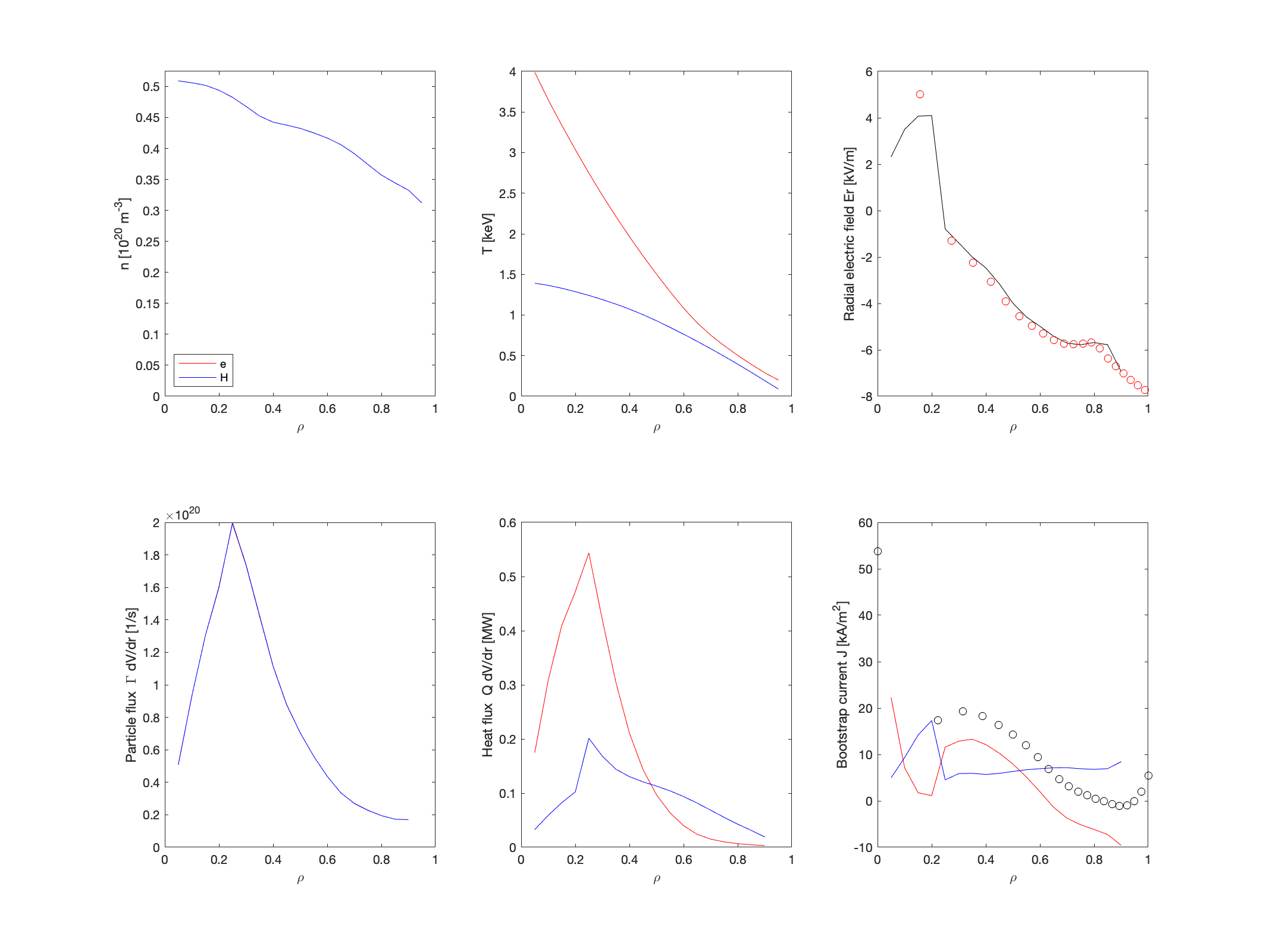
% load Json
    fid=fopen(cooker_file);
    str=fgetl(fid);
    fclose(fid);
    prof_data=jsondecode(str);
    % Define profile functions based on cooker data
    rho_vmec = 0:0.05:1;
    s_vmec = rho_vmec.*rho_vmec;
    f_te = @(s) max(pchip((prof_data.thomson_Te.reff./max(prof_data.thomson_Te.reff)).^2,...
        prof_data.thomson_Te.value.*1E3,s),0);
    f_ne = @(s) max(pchip((prof_data.thomson_ne.reff./max(prof_data.thomson_ne.reff)).^2,...
        prof_data.thomson_ne.value.*1E19,s),0);
    f_ti = @(s) max(pchip((prof_data.cxrs_Ti.reff./max(prof_data.cxrs_Ti.reff)).^2,...
        prof_data.cxrs_Ti.value.*1E3,s),0);
    dfds_te = @(s) (f_te(s+1E-6)-f_te(s-1E-6))./2E-6;
    dfds_ti = @(s) (f_ti(s+1E-6)-f_ti(s-1E-6))./2E-6;
    dfds_ne = @(s) (f_ne(s+1E-6)-f_ne(s-1E-6))./2E-6;
    % Setup some values based on conf_name
    switch conf_name
        case 'EIM'
            equilID = 'w7x-sc1';
            extcur_conf=[13400*108  13400*108  13400*108  13400*108  13400*108  0*36  0*36];
        case 'KJM'
            equilID = 'w7x-hm1';
            extcur_conf=[13130*108  12760*108  12150*108  11550*108  11180*108  0*36  0*36];
        case 'FTM'
            equilID = 'w7x-schi';
            extcur_conf=[14188*108 14188*108 14188*108 14188*108 14188*108 -9790*36 -9790*36];
        case 'DBM'
            equilID = 'w7x-scli';
            extcur_conf=[11769*108 11769*108 11769*108 11769*108 11769*108 8827*36 8827*36];
        otherwise
            disp('Please choose conf_name to be: EIM, KJM, FTM, DBM');
            return;
    end
    % Define profiles for NEOTRANSP
    h0=0.05;
    rho=h0:h0:(1-h0);
    s=rho.*rho;
    Prof=[];
    %Electrons
    Prof(1).Z=-1;
    Prof(1).TkeV=f_te(s).*1E-3;
    Prof(1).dTkeVdrho=dfds_te(s).*1E-3.*2.*rho;
    Prof(1).n20=f_ne(s).*1E-20;
    Prof(1).dn20drho=dfds_ne(s).*1E-20.*2.*rho;
    %Ions
    Prof(2).Z=1;
    Prof(2).m_au=1;
    Prof(2).TkeV=f_ti(s).*1E-3;
    Prof(2).dTkeVdrho=dfds_ti(s).*1E-3.*2.*rho;
    Prof(2).n20=f_ne(s).*1E-20;
    Prof(2).dn20drho=dfds_ne(s).*1E-20.*2.*rho;
    % Neotransp options
    Opt.makeErsearchplot=0; %set to 0 to turn off, or to the figure number
    Opt.roots='i/e';          %can be 'i', 'e', 'i&e'
    Opt.surfInterpVar = 'rho'; % r/a not W7AS r
    % Run Neotransp
    Transp= neotransp(equilID,rho,Prof,B00axis,Opt);
    % Calculate bootstrap profile and CURTOR
    jboot = squeeze(Transp.Bootstrapcurrdens.i)+squeeze(Transp.Bootstrapcurrdens.e)';
    jboot(isnan(jboot)) = 0;
    jboot_spl = spline(rho,jboot);
    Itor = sum(jboot.*Transp.dVds'.*h0./(2.*pi.*Transp.R00'));
    % Calculate Phi_estatic for BEASM3D
    dphi=Transp.dPhidskV.*1E3; % kV to V
    sh = 0.5.*(s(2:end)+s(1:end-1)); %half grid
    f =(dphi(2:end)+dphi(1:end-1)).*0.5; %half grid
    phi = cumsum(f.*diff(s))+dphi(1);
    % Make NEOSTRANSP plot
    pp = pchip(sqrt(sh),phi);
    h3 = 0.05;
    s3 = 0:h3:1;
    rho3=sqrt(s3);
    plottransp(Transp); set(gcf,'Position',[1 1 1024 768],'Color','white');
    drawnow;
    subplot(2,3,6); hold on; f=ppval(jboot_spl,rho3); plot(rho3,f./1E3,'ok');
    subplot(2,3,3); hold on; f=ppval(pp,rho3); x=0.5.*(s3(2:end)+s3(1:end-1)); dphids=-diff(f)./diff(s3); Er=dphids.*sqrt(x).*2./Transp.minorradiusW7AS./1E3; plot(sqrt(x),Er,'or');
    saveas(gcf,['transp_' outfile '.fig']);
    saveas(gcf,['transp_' outfile '.png']);
    close(gcf);
    % Write NEOTRANSP Profiles to file
    fid = fopen(['transp_' outfile '.txt'],'w');
    fprintf(fid,'#r/a #ne [m^-3] #ni1 [m^-3] #te [eV] #ti1 [eV] #dPhi/ds [V] #jboot [A/m^2] #Gamma_e [1/s] #Gamma_i1 [1/s] #Q_e [W] #Q_i1 [W]\n');
    for i=1:length(rho)
        fprintf(fid,'%20.10E %20.10E %20.10E %20.10E %20.10E %20.10E %20.10E %20.10E %20.10E %20.10E %20.10E\n',...
            rho(i),Transp.Prof(1).n20(i).*1E20,Transp.Prof(2).n20(i).*1E20,Transp.Prof(1).TkeV(i).*1E3,Transp.Prof(2).TkeV(i).*1E3,...
            Transp.dPhidskV(i).*1E3,Transp.Bootstrapcurrdens.i(1,1,i)+Transp.Bootstrapcurrdens.e(1,i),...
            Transp.Flux.e(1,i),Transp.Flux.i(1,1,i),Transp.Heatflux.e(1,i).*1E6,Transp.Heatflux.i(1,1,i).*1E6);
    end
    fclose(fid);
    % Setup input
    ec = 1.60217662E-19;
    p_vmec = f_ne(s_vmec).*ec.*(f_te(s_vmec)+f_ti(s_vmec)./zeff);
    j_vmec = ppval(jboot_spl,rho_vmec);
    boundary = get_w7x_fixedboundary([conf_name num2str(round(B00axis.*100),'%+3.3i')],[],[],[],[],[],[]);
    vmec_input = vmec_namelist_init_w7x('INDATA');
    vmec_input.ns_array=[16 32 64 128];
    vmec_input.ftol_array=[1E-30 1E-30 1E-30 1E-12];
    vmec_input.niter_array=[1000 2000 4000 20000];
    vmec_input.nstep=200; vmec_input.delt=1; vmec_input.tcon0=1; vmec_input.niter=20000;
    vmec_input.gamma=0; vmec_input.bloat=1; vmec_input.spres_ped=1; vmec_input.pres_scale=1;
    vmec_input.pmass_type='akima_spline';
    vmec_input.am_aux_s=s_vmec;
    vmec_input.am_aux_f=p_vmec;
    vmec_input.ncurr=1; vmec_input.pcurr_type='akima_spline_ip'; vmec_input.curtor=Itor;
    vmec_input.ac_aux_s=s_vmec;
    vmec_input.ac_aux_f=j_vmec;
    vmec_input.nfp = 5;
    vmec_input.mpol = 13;
    vmec_input.ntor = 10;
    vmec_input.nzeta=24;
    vmec_input.ntheta=32;
    vmec_input.lfreeb=0;
    vmec_input.extcur=-extcur_conf;
    vmec_input.datatype='VMEC_input';
    vmec_input.phiedge=boundary.phiedge;
    vmec_input.xm=boundary.xm;
    vmec_input.xn=boundary.xn;
    vmec_input.rbc=boundary.rbc;
    vmec_input.zbs=boundary.zbs;
    dexm=boundary.xm==0;
    vmec_input.raxis=boundary.rbc(dexm);
    vmec_input.zaxis=boundary.zbs(dexm);
    vmec_input=rmfield(vmec_input,'bcrit');
    % Now write input file
    filename=['input.' outfile];
    write_vmec_input_w7x(filename,vmec_input);
    w7x_beam_params(1:8,'H2','write_beams3d','TE',[s_vmec;f_te(s_vmec)],...
        'NE',[s_vmec;f_ne(s_vmec)],'TI',[s_vmec;f_ti(s_vmec)],...
        'ZEFF',[s_vmec; 0.*s_vmec+zeff],...
        'POT',[s3;ppval(pp,rho3)],'file',filename,'t_end',0.100,...
        'NPOINC',3,'nphi',72);
The equilibrium w7x-sc1 is in the database. Taking the DKES data from there.
    Performing Er search
    rho=0.050, residule: e0.0047, : iInf, e0.0047
    rho=0.100, residule: e0.0142, e0.0002, : iInf, e0.0002
    rho=0.150, residule: i0.1411, e0.0150, i0.1240, e0.0016, i0.1538, e0.0000, i0.0801, e0.0000, i0.0513, e0.0000, i0.0351, e0.0000, i0.0249, e0.0000, i0.0181, e0.0000, i0.0134, e0.0000, i0.0100, e0.0000, i0.1585, e0.0008, i0.0882, e0.0004, i0.0399, e0.0002, i0.0101, e0.0001, i0.0000, e0.0000, : i0.0000, e0.0000
    rho=0.200, residule: i0.0150, e0.0302, i0.0022, e0.0027, : i0.0022, e0.0027
    rho=0.250, residule: i0.0808, i0.0024, : i0.0024, eInf
    rho=0.300, residule: i0.0823, i0.0119, i0.0018, : i0.0018, eInf
    rho=0.350, residule: i0.0559, i0.0105, i0.0025, : i0.0025, eInf
    rho=0.400, residule: i0.0352, i0.0074, i0.0014, : i0.0014, eInf
    rho=0.450, residule: i0.0202, i0.0015, : i0.0015, eInf
    rho=0.500, residule: i0.0135, i0.0002, : i0.0002, eInf
    rho=0.550, residule: i0.0057, i0.0000, : i0.0000, eInf
    rho=0.600, residule: i0.0108, i0.0001, : i0.0001, eInf
    rho=0.650, residule: i0.0104, i0.0001, : i0.0001, eInf
    rho=0.700, residule: i0.0016, : i0.0016, eInf
    rho=0.750, residule: i0.0035, : i0.0035, eInf
    rho=0.800, residule: i0.0222, i0.0003, : i0.0003, eInf
    rho=0.850, residule: i0.0440, i0.0005, : i0.0005, eInf
    rho=0.900, residule: i0.0390, i0.0005, : i0.0005, eInf
    rho=0.950, residule:
    Warning: All NaN entries in the first and second input were ignored.
       Configuration: EIM+252